Monte Carlo methods and Application to Ising Model
            Yingjie Wang

            Apr. 19,  2022
1. Introduction to the Monte Carlo Method
1.1 Background
What's the problem?
- In canonical ensemble, everything can be calculated from: $$Z = \operatorname{tr}\left(\mathrm{e}^{- \beta \hat{H}}\right) = \sum_{s} \mathrm{e}^{- \beta E_s},$$
- but it's hard to calculate in general!
- You may say that, OK let's do that numerically, but running over the states is still hard
What's Monte Carlo Method?
It's hard to define generally...
Here we refer to the Metropolis Monte Carlo Algorithm, which will be defined later.
How Monte Carlo Solve the problem?
- Every quantity can be calculated by $$\left\langle A\right\rangle = \sum_s A(s) \frac{\mathrm{e}^{-\beta E_s}}{Z},$$ so we can randomly select states according to the probability $$p(s) = \frac{\mathrm{e}^{-\beta E_s}}{Z}$$ and calculate the average on the sample states, instead of run over all states
- The point is: overall constant factor is not matter in the Metropolis algorithm!
- Knowing that $$p(s) \propto \mathrm{e}^{- \beta E_s}$$ is enough. Good News!
1.2 The Metropolis algorithm
Suppose that we want a dataset $\{ x_i \}$ that match some probability distribution $p(x)$.
- Start from any initial value $x_0$;
- Do the following loop:
- suppose we already have $x_i$. Move to a test value $x^{\prime}_{i+1}$ for $x_{i+1}$ randomly from $x_i$ according to any symmetric distribution $T(x_{i+1},x_i)$ (but must make sure that $x^{\prime}_{i+1} \neq x_i$);
- accept the change according to the probability $A(x^\prime_j,x_i) = \min(1, p(x^\prime_j)/p(x_i))$. If we accept the move, then $x_{i_1} = x^\prime_{i+1}$; else we throw $x^\prime_j$ and take $x_{i+1} = x_i$. Note that the algorithm only depends on $p(y)/p(x)$, any overall factor doesn't matter!
- After many loops, the distribution of $\{ x_i \}$ will converge to $\propto p(x)$.
- Then throw all $x_i$ generated before, just leave the last one, then do more loops to collect enough samples.
Example: coding time
import numpy as np
from matplotlib import pyplot as plt
rng = np.random.default_rng()
def p(x):
	return np.exp(-x*x/2)
def metro_norm(stepnum: int, dx: float) -> np.array:
	x = np.empty(stepnum)
	x[0] = -10
	for i in range(stepnum-1):
		y = x[i] + (rng.random()-0.5)*dx
		if rng.random() < p(y)/p(x[i]):
			x[i+1] = y
		else:
			x[i+1] = x[i]
	return x
xlist = metro_norm(10000,0.5)
# plot
plt.subplot(2, 2, 1)
plt.scatter(range(10000),xlist,s=1)
plt.subplot(2, 2, 2)
plt.hist(xlist[3000:],density=True)
plt.plot(np.arange(-3,3,step=0.1),p(np.arange(-3,3,step=0.1))/np.sqrt(2*np.pi))
%config InlineBackend.figure_format='svg'
plt.show()

only 10000 run in $0.6 s$, but still not bad, right?
2 Metropolis algorithms for statistical mechanics
2.1 In canonical ensemble
$x_i \rightarrow s_i, \ p(x_i) \rightarrow p(s_i) = \mathrm{e}^{-\beta E}$
The accepting probability is now $p(s_j)/p(s_i) = \mathrm{e}^{- \beta \Delta E}$
- Everything is almost the same, do loops to generate a list of states.
- Calculate $\left< A \right>$ on the sample list
Toy model: Ideal gas
- Suppose that we have $N$ particles in $V=L^3$ box.
- For each particle, the energy eigenstates are $\left| \vec{n} \right> = \left| n_1 \right>\left| n_2 \right>\left| n_3 \right>$ with the eigenvalue $E_{\vec{n}} = \frac{\pi^2 \hbar^2}{2mL^2} \left( n_1^2 + n_2^2 + n_3^2 \right)$.
- Take $\hbar = m = L = k = 1$ for convenient.
- The steps:
- We create a list
nwith shape $N \times 3$ to present the state. - Randomly choose one particle $i \in [0,N-1]$ and one direction $j \in [0,2]$, then randomly add $\pm 1$ to
n[i,j] - The change of energy is $\Delta E = \frac{\pi^2}{2} (\pm 2 n_{i,j} + 1)$
- If
rand()$< \mathrm{e}^{- E/T}$, then accept the move. Otherwise, keepn[i,j]unchanged. - Let the computer repeat!
- We create a list
The code
from rich.progress import track
def elist(T, N=1000, movenum = 2000000):
	energy = np.pi*np.pi*3*N/2
	nlist = np.ones((N,3))
	energylist = np.empty(movenum)
	for move in track(range(movenum)):
		i,j = rng.integers(N),rng.integers(3)
		x = rng.integers(2)
		if x == 1 or nlist[i,j] > 1:
			dE = (2*nlist[i,j]*(2*x-1) + 1)*np.pi*np.pi/2
			if rng.random() < np.exp(-dE/T):
				nlist[i,j] += 2*x - 1
				energy += dE
		energylist[move] = energy
	return energylist/N
data = elist(1000)
plt.plot(data)
plt.show()
Output()

Vectorized code
def e_vec(T, N=1000, movenum = 1000000):
	NT = T.size
	energy = np.pi*np.pi*3*N/2
	nlist = np.ones((N,3,NT))
	energylist = np.empty((movenum, NT))
	for move in track(range(movenum)):
		i,j = rng.integers(N),rng.integers(3)
		x = rng.integers(2)
		validlist = ([x == 1] | (nlist[i,j] > 1))
		dE = (2*nlist[i,j]*(2*x-1) + 1)*np.pi*np.pi/2
		boollist = rng.random() < np.exp(-dE/T)
		nlist[i,j] += (2*x - 1)*validlist*boollist
		energy += dE*validlist*boollist
		energylist[move] = energy
	elist = np.mean(energylist[movenum//2:],axis=0)
	return elist/N
tlist = np.arange(100,1000)
elist = e_vec(tlist)
plt.scatter(tlist,elist, s=1)
plt.show()
Output()

When $T$ is a large number (prepare to $\frac{\hbar^2}{kmL^2}$), $e(T)$ recover the straight line $e = \frac{3}{2} T$.
3 Ising model
Now let's apply the MC method to a specific system. Here I take Ising model for example.
What's it for?
Ising model is used to explain ferromagnet.

Questions:
- Why $M \neq 0$ when $\vec{B} = 0$ and $T$ is lower than some value
- Why there's a critical temperature
- ...
What's Ising model's answer
In most ordinary materials the magnetic dipoles of the atoms have a random orientation. In effect this non-specific distribution results in no overall macroscopic magnetic moment. However in certain cases, such as iron, a magnetic moment is produced as a result of a preferred alignment of the atomic spins.
Ising model suppose that there's a short-range interaction term in the Hamiltonian: $$H = - J \sum_{<i,j>} \sigma_{i} \sigma_j - B \sum_i \sigma_i, \quad J>0,$$ where $\sum_{<i,j>}$ means that sum over nearby spin pairs, and $\sigma$ is the $z$-direction spin operator.
But since $\sigma_i$ commute with each other, the Hamiltonian just acts as number. We will treat this model as a "classical" system and treat $\sigma_i$ as a variable taking it's value of $\pm 1$.
The existing of $J$ term can explain the difference between ferromagnetism behavior and paramagnetism behavior.
3.1 Ising model on 2D finite square lattice
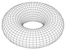
We introduce the periodic boundary condition on a $N \times N$ lattice, so that each spin always interacts with 4 spins.
Thus the model is defined on a torus.
We'll also assuming that $ B = 0, \quad J=1$.
3.1.1 the Analytical Solution
Just post to show it...
I get the partition function using mathematica for $N=8$ lattice:
$$ Z(\beta) = \mathrm{e}^{2N^2 \beta} \tilde{Z}(\mathrm{e}^{-2 \beta}),$$ where $\tilde{Z}(x)$ is a polynomial:
$$ \tilde{Z}(x) = 2 x^{128}+128 x^{124}+256 x^{122}+4672 x^{120}+17920 x^{118}+145408 x^{116}+712960 x^{114}+4274576 x^{112}+22128384 x^{110}+118551552 x^{108}+610683392 x^{106}+3150447680 x^{104}+16043381504 x^{102}+80748258688 x^{100}+396915938304 x^{98}+1887270677624 x^{96}+8582140066816 x^{94}+36967268348032 x^{92}+149536933509376 x^{90}+564033837424064 x^{88}+1971511029384704 x^{86}+6350698012553216 x^{84}+18752030727310592 x^{82}+50483110303426544 x^{80}+123229776338119424 x^{78}+271209458049836032 x^{76}+535138987032308224 x^{74}+941564975390477248 x^{72}+1469940812209435392 x^{70}+2027486077172296064 x^{68}+2462494093546483712 x^{66}+2627978003957146636 x^{64}+2462494093546483712 x^{62}+2027486077172296064 x^{60}+1469940812209435392 x^{58}+941564975390477248 x^{56}+535138987032308224 x^{54}+271209458049836032 x^{52}+123229776338119424 x^{50}+50483110303426544 x^{48}+18752030727310592 x^{46}+6350698012553216 x^{44}+1971511029384704 x^{42}+564033837424064 x^{40}+149536933509376 x^{38}+36967268348032 x^{36}+8582140066816 x^{34}+1887270677624 x^{32}+396915938304 x^{30}+80748258688 x^{28}+16043381504 x^{26}+3150447680 x^{24}+610683392 x^{22}+118551552 x^{20}+22128384 x^{18}+4274576 x^{16}+712960 x^{14}+145408 x^{12}+17920 x^{10}+4672 x^8+256 x^6+128 x^4+2 $$
OK, I think you already don't want to see any more equation like this, let's move to the MC method...
3.1.2 Python Time
- Use a table
s[i,j]to save spins; - Set any initial state;
- Randomly choose
i,jto flip the spin; - $\Delta E = -J(\text{nearby sum}) \times \Delta s_{ij} = 2J(\text{nearby sum})*s_{ij}$;
- When
random()${}< \mathrm{e}^{-\Delta E/T}$, accept the flip; - Let the computer repeat!
Test
def gqlist(N):
	if N==2:
		return [2, 0, 12, 0, 2]
	elif N== 4:
		return [2,0,32,64,424,1728,6688,13568,20524,13568,6688,1728,424,64,32,0,2]
	elif N== 8:
		return [2, 0, 128, 256, 4672, 17920, 145408, 712960, 4274576, 22128384, 118551552, 610683392, 3150447680, 16043381504, 80748258688, 396915938304, 1887270677624, 8582140066816, 36967268348032, 149536933509376, 564033837424064, 1971511029384704, 6350698012553216, 18752030727310592, 50483110303426544, 123229776338119424, 271209458049836032, 535138987032308224, 941564975390477248, 1469940812209435392, 2027486077172296064, 2462494093546483712, 2627978003957146636, 2462494093546483712, 2027486077172296064, 1469940812209435392, 941564975390477248, 535138987032308224, 271209458049836032, 123229776338119424, 50483110303426544, 18752030727310592, 6350698012553216, 1971511029384704, 564033837424064, 149536933509376, 36967268348032, 8582140066816, 1887270677624, 396915938304, 80748258688, 16043381504, 3150447680, 610683392, 118551552, 22128384, 4274576, 712960, 145408, 17920, 4672, 256, 128, 0, 2]
def E_theory(T,N=16):
	x = np.exp(-2/T)
	Ztitle = 0
	glist = gqlist(N)
	for i in range(N*N+1):
		Ztitle += glist[i]*np.power(x,2*i)
	thE = 0
	for i in range(N*N+1):
		thE += i*(glist[i]*np.power(x,2*i)/(Ztitle*N*N))
	thE *= 4
	thE -= 2
	return thE
from rich.progress import track
from rich.console import Console
from rich.table import Table
def Ising2D_E(T,moves,N=16):
	J = 1
	B = 0

	slist = np.ones((N,N), dtype=int)
	energylist = np.empty(moves)
	energy = - 2*J * N * N
	acp = 0

	for step in track(range(moves)):
		[i,j] = rng.integers(N,size=2)
		dE = 2*J*(slist[(i-1)%N,j] + slist[(i+1)%N,j] + slist[i,(j-1)%N] + slist[i,(j+1)%N])*slist[i,j]
		if rng.random() < np.exp(-dE/T):
			acp += 1
			slist[i,j] *= -1
			energy += dE
		energylist[step] = energy
	eth = E_theory(N=N,T=T)
	emc = np.mean(energylist[moves//2:])/(N*N)

	table = Table(title="energy of 2D Ising")
	table.add_column("T", style = "green")
	table.add_column("theoretical", style="cyan")
	table.add_column("Monte Calor", style="magenta")
	table.add_column("persentage error", style = "blue")
	table.add_row(str(T),str(eth), str(emc), str(100*(emc-eth)/eth)+"%")

	console = Console()
	console.print(table)
	return energylist/(N*N)
elist = Ising2D_E(5, 100000, N=8)
plt.plot(elist)
%config InlineBackend.figure_format='svg'
plt.show()
Working... ━━━━━━━━━━━━━━━━━━━━━━━━━━╸━━━━━━━━━━━━━ 67% 0:00:01
                       energy of 2D Ising
┏━━━┳━━━━━━━━━━━━━━━━━━━━━┳━━━━━━━━━━━━━┳━━━━━━━━━━━━━━━━━━━━━━┓
┃ T ┃ theoretical         ┃ Monte Calor ┃ persentage error     ┃
┡━━━╇━━━━━━━━━━━━━━━━━━━━━╇━━━━━━━━━━━━━╇━━━━━━━━━━━━━━━━━━━━━━┩
│ 5 │ -0.4283680589440815 │ -0.41901625 │ -2.1831247098893214% │
└───┴─────────────────────┴─────────────┴──────────────────────┘

(1) Energy
from scipy.stats import chi2,halfnorm,t

def Ising2D_E_vec(T,moves,N=16):
	J = 1
	B = 0
	NT=T.size

	slist = np.ones((N,N,NT), dtype=int)
	energylist = np.empty((moves,NT))
	energy = - 2*J * N * N

	for step in track(range(moves)):
		[i,j] = rng.integers(N,size=2)
		dE = 2*J*(slist[(i-1)%N,j] + slist[(i+1)%N,j] + slist[i,(j-1)%N] + slist[i,(j+1)%N])*slist[i,j]
		boollist = rng.random() < np.exp(-dE/T)
		slist[i,j] *= 1-2*boollist
		energy += dE*boollist
		energylist[step] = energy
	validElist = energylist[moves//2:]/(N*N)
	emc = np.mean(validElist,axis=0)
	S=np.std(validElist, ddof=1, axis=0)
	halfn = validElist.size
	errbar = S*t.isf(0.05,halfn-1)/np.sqrt(halfn)
	return emc,errbar
N = 8
T=np.arange(0.5, 5, step=0.1)
N=8
elist, errbar = Ising2D_E_vec(T, 200000, N=N)
if N in [2,4,8]:
	thElist = E_theory(T,N=N)
	plt.plot(T,thElist)
plt.errorbar(T, elist, yerr=errbar, fmt="None")
plt.scatter(T,elist, marker="x", c="r", zorder=2.5)
plt.title("E/N^2 vs T")
plt.show()
Output()

(2) Magnetization $M$
$$ M = \left< \sum_i \sigma_i \right> $$
from scipy.stats import chi2,halfnorm,t
def Ising2D_M_vec(T,moves=1000000, N=16):
	J = 1
	B = 0
	NT=T.size

	slist = np.ones((N,N,NT), dtype=int)
	Mlist = np.empty((moves, NT))
	M = N*N

	for step in track(range(moves)):
		[i,j] = rng.integers(N,size=2)
		dE = 2*J*(slist[(i-1)%N,j] + slist[(i+1)%N,j] + slist[i,(j-1)%N] + slist[i,(j+1)%N])*slist[i,j]
		boollist = rng.random() < np.exp(-dE/T)
		slist[i,j] *= 1-2*boollist
		M += 2*slist[i,j]*boollist
		Mlist[step] = M
	# eth = -J*(1+2*(2*(np.tanh(2*J/T)**2)-1)*ellipk(2*np.tanh(2*J/T)/np.cosh(2*J/T)))/np.tanh(2*J/T)
	validMlist = Mlist[moves//2:]/(N*N)
	Mmc = np.mean(validMlist,axis=0)
	S=np.std(validMlist, ddof=1, axis=0)
	halfn = validMlist.size
	errbar = S*t.isf(0.00135,halfn-1)/np.sqrt(halfn)
	return Mmc,errbar
T=np.arange(0.5, 5, step=0.1)
Tt= np.arange(0.5,5,step = 0.02)
N=16
Mlist, errbar = Ising2D_M_vec(T, 1000000, N=N)
a = 1-np.power(np.sinh(2/Tt),-4)
thMlist = np.power(a*(a>0),1/8)
plt.plot(Tt,thMlist)
plt.errorbar(T, Mlist, yerr=errbar, marker="x")
plt.title("M/N^2 vs T")
plt.show()
Output()

Metropolis MC method works not very well around the critical temp!
(3) heat capacity $C$
$$ C = \frac{\partial \left< E \right>}{\partial T} = \frac{(\Delta E)^2}{T^2} $$
from scipy.stats import chi2,halfnorm,t
def Ising2D_C_vec(T,moves=1000000,N=16):
	J = 1
	B = 0
	NT=T.size

	slist = np.ones((N,N,NT), dtype=int)
	energylist = np.empty((moves,NT))
	energy = - 2*J * N * N

	for step in track(range(moves)):
		[i,j] = rng.integers(N,size=2)
		dE = 2*J*(slist[(i-1)%N,j] + slist[(i+1)%N,j] + slist[i,(j-1)%N] + slist[i,(j+1)%N])*slist[i,j]
		boollist = rng.random() < np.exp(-dE/T)
		slist[i,j] *= 1-2*boollist
		energy += dE*boollist
		energylist[step] = energy
	validElist = energylist[moves//2:]/(N*N)
	halfn = validElist.size
	S=np.std(validElist, ddof=1, axis=0)
	cmc = S*S/(T*T)
	alpha = 0.01
	c1 =chi2.isf(alpha/2, halfn - 1)
	c2 = chi2.isf(1-alpha/2, halfn - 1)
	errbar = np.array([(1-(halfn - 1)/c1)*cmc,((halfn-1)/c2 - 1)*cmc])
	return cmc,errbar
T = np.arange(0.5, 10,step=0.2)
C,errbar = Ising2D_C_vec(T)
plt.errorbar(T, C, yerr=errbar, marker="x")
plt.title("C0 vs T")
plt.show()
Output()

(4) susceptibility $\chi$
$$ \chi=\frac{\partial M}{\partial T}=\frac{(\Delta M)^{2}}{T}=\frac{\langle M^{2}\rangle-\langle M\rangle^{2}}{T} $$
from scipy.stats import chi2
def Ising2D_chi_vec(T,moves=1000000,N=16):
	J = 1
	B = 0
	NT=T.size

	slist = np.ones((N,N,NT), dtype=int)
	Mlist = np.empty((moves,NT))
	M = J * N * N

	for step in track(range(moves)):
		[i,j] = rng.integers(N,size=2)
		dE = 2*J*(slist[(i-1)%N,j] + slist[(i+1)%N,j] + slist[i,(j-1)%N] + slist[i,(j+1)%N])*slist[i,j]
		boollist = rng.random() < np.exp(-dE/T)
		slist[i,j] *= 1-2*boollist
		M += 2*slist[i,j]*boollist
		Mlist[step] = M
	validMlist = Mlist[moves//2:]/(N*N)
	halfn = validMlist.size
	S=np.std(validMlist, ddof=1, axis=0)
	chimc = S*S/t
	alpha = 0.01
	c1 =chi2.isf(alpha/2, halfn - 1)
	c2 = chi2.isf(1-alpha/2, halfn - 1)
	errbar = np.array([(1-(halfn - 1)/c1)*chimc,((halfn-1)/c2 - 1)*chimc])
	return chimc,errbar
T = np.arange(0.5, 6,step=0.2)
chi,errbar = Ising2D_chi_vec(T)
plt.errorbar(T, chi, yerr=errbar, marker="x")
plt.title("chi vs T")
plt.show()
Working... ━━━━━━━━━━━━━━━━━━━━━━━━━━━━━━━━━━━━━━━━ 0% -:--:--

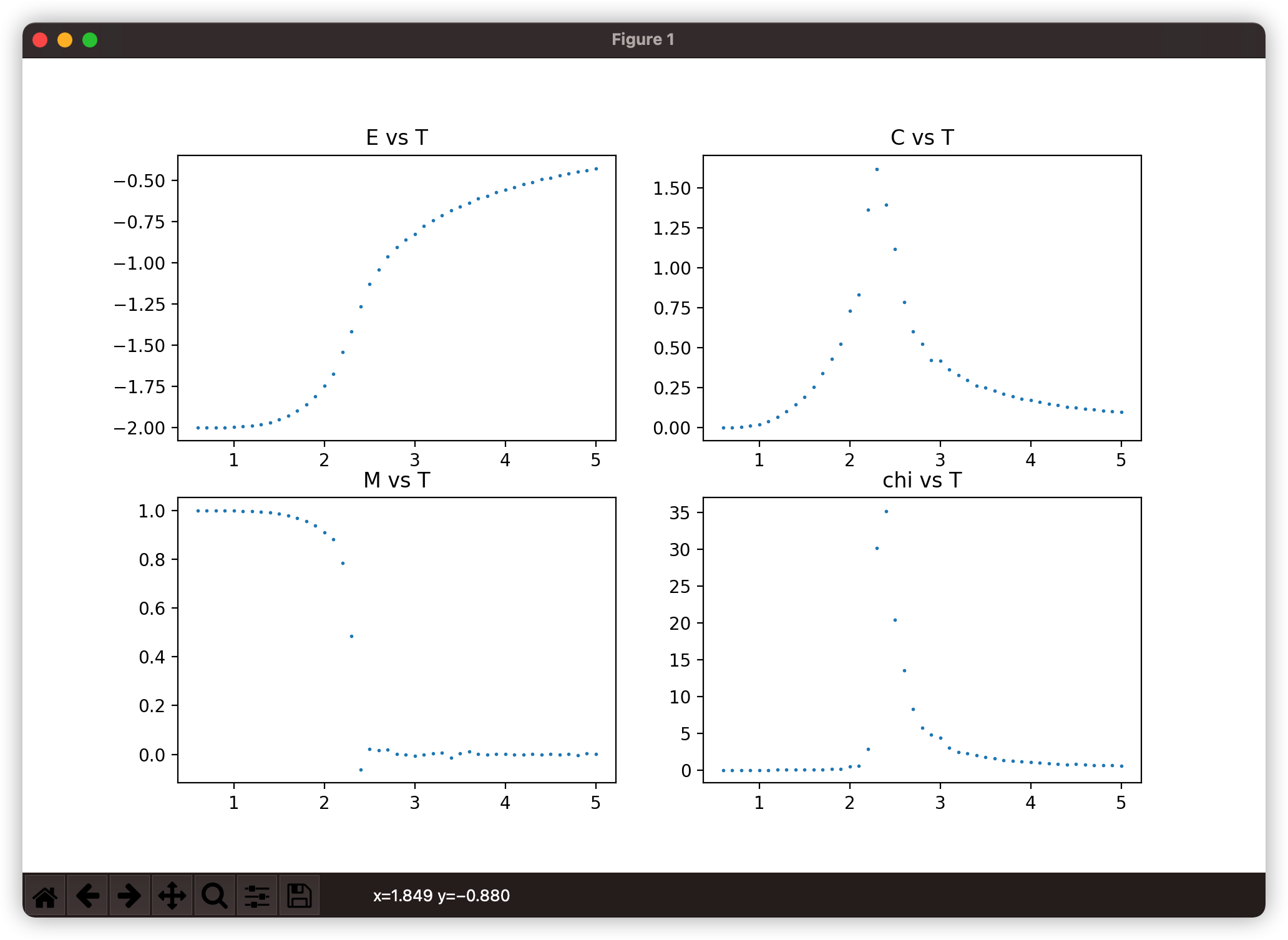
Run over T
Let $T$ vary slowly from high to low.
# Ising2D_runover_T.py
# too long to show...
Run over $B$
We relax the $B=0$ condition, and fix $T=1$ (low temperature) --- Just like magnetize an iron block!
# run external Ising2D_runover_B.py
%config InlineBackend.figure_format='svg'
import Ising2D_runover_B
Output()

We can see the path dependence!
Conclusion
- The Metropolis MC is very fast
- It's also accuracy, except $T \sim T_c$
- The code can be easily reuse for another quantity
- Depends on:
rng, random number generator- a good step $\Delta x$